Welcome to my Stock Market Analysis Project!

I completed this project as a walk-through project during one of my courses. As my interest grew, I made great additions in the code using python as well as Tableau. Here is a brief summary of what I have done.

Here’s what I’ve done so far -

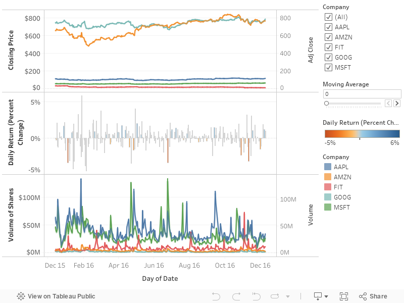
Here is the an overview of the data in this Tableau Dashboard

And this Jupyter Notebook contains my data exploration, analysis and visualization work for the project.

A template for time series analysis on the shares’ data on any company.

Here is an example for Ford Motors

The data fetched is from yahoo for the last 15 years

Close

Closing prices are stationary

First Difference

We can consider analyzing a first difference of the series. value of (t-1) is subtracted from value of (t).

First difference is relatively stationary and mostly fluctuates around 0. But variance of this series can vary over time. We need to incorporate mechanism to accomodate for sensing smaller variances along with the larger ones. Hence, Log.

Log

Log of closing price

So that gives us the original closing price with a log transform applied to “flatten” the data from an exponential curve to a linear curve. One way to visually see the effect that the log transform had is to analyze the variance over time. We can use a rolling variance statistic and compare both the original series and the logged series.

Variance - with and without Log

Normal and Logged First Difference

Create a few more lag variables

Now we create a few more lab variables with lag of 1, 2, 5 and 30 days

No apparent Correlation. It means that today’s index values does not tell much about at least a few days in the future.

Lag relationships

There could be relation in the values we did not try. There is a function to test those relationships. Let’s try those.

Seasonal Decomposition

ARIMA analysis

Analyis for perfomed, but as expected, it yielded inaccurate predictions. (Predicting shared ain’t that easy!)